TL;DR for Busy Engineers

If you're running an ML feature store or any large-scale analytics pipeline that reads Parquet files from cloud storage, you're probably leaving 50-90% performance on the table without touching your compute infrastructure. We achieved:

• 78% faster reads on 200M+ record metric datasets (DuckDB)
• 89% faster reads on 28M+ record event datasets (DuckDB)
• Up to 97% reduction in complex feature engineering workloads
• 16-47% file size reduction across different data types
• Zero additional infrastructure cost
• No memory footprint increase

The secret? Three Parquet export optimizations that most teams overlook: column typing and compression, data sorting, and file sizing with smart partitioning. We show Snowflake examples below, but the principles apply to any OLAP system exporting to Parquet (BigQuery, Redshift, Databricks, etc.)

What you'll learn: ‍

• The three critical Parquet optimizations that delivered 50-97% performance gains from defaults
• Production-grade architecture decisions for SOC2-compliant, multi-tenant ML infrastructure
• DuckDB vs Polars performance characteristics and why identical optimizations affected them differently
• Real-world benchmarking methodology using 200M+ healthcare records on AWS EKS and Fargate
• Complete implementation guide with SQL examples and Python benchmarking scripts

What you'll also discover:‍

• How we architected a SOC2-compliant, multi-tenant feature store on Kubernetes with complete client data isolation
• The infrastructure stack (Dagster, EKS, Terraform) that makes this scale to thousands of concurrent jobs
• Production validation metrics showing job duration improvements without memory overhead

Read on for the full story—or skip to the Implementation Checklist if you're already sold.

The Problem We Didn't Know We Had

Here's a story that might sound familiar.

Our ML platform at ODAIA powers a feature store that processes billions of records across multiple enterprise clients. Like many teams, we evolved our architecture organically, adding features, scaling out, and occasionally throwing more compute at problems when things got slow.

The architecture looked reasonable on paper: data warehouse exports to S3 as Parquet files, with DuckDB and Polars handling feature computation on those files. Simple enough.

Then we started noticing the symptoms.

Query queues that never seemed to clear. Our single analytics warehouse was handling developer queries, scheduled exports, and pipeline runs simultaneously. When export jobs kicked off, everything else ground to a halt.

The knee-jerk reaction? Spin up a larger warehouse. Throw more credits at the problem.

But here's the thing—that's not engineering, that's avoidance.

We decided to dig deeper. What we found changed how we think about data export entirely.

Why We Built Our Feature Store This Way

Before diving into the solution, it's worth explaining why our architecture was designed the way it was. This isn't just a story about Parquet optimization—it's about building a secure, scalable ML platform for enterprise healthcare clients.

The Architecture Decision: Snowflake to S3

Why export data from Snowflake to S3 instead of computing features directly in Snowflake?

1. Massive Parallelization

Our feature generation process runs thousands of concurrent jobs during each computation cycle. Each job computes different feature sets, rolling windows, lag features, behavioural aggregations, and more across multiple client datasets.

Running this in Snowflake would require scaling to expensive warehouse tiers. By exporting to S3 and computing with DuckDB and Polars on Kubernetes (EKS), we achieve horizontal scalability at a fraction of what it would cost in Snowflake credits.

2. Cost Efficiency

Snowflake charges for compute time. A single large warehouse running complex feature engineering for hours gets expensive fast. Our approach:

• Use Snowflake for what it's best at: reliable, ACID-compliant data warehousing
• Export once to S3 (cheap storage)
• Compute features on ephemeral Kubernetes pods (pay only for what you use)

3. Compute-Storage Decoupling

By separating storage (S3) from compute (Kubernetes), we can scale each independently. Need more compute? Spin up more pods. Need more storage? S3 scales infinitely. Neither depends on the other.

Infrastructure Stack

Our feature store runs on a modern, cloud-agnostic infrastructure stack:

This stack is portable by design. While we currently run on AWS, the architecture doesn't have hard dependencies on AWS-specific services. Dagster, Kubernetes, and Terraform work across cloud providers.

Multi-Tenant Security: Data Isolation by Design

Here's where security becomes non-negotiable. We serve multiple enterprise healthcare clients, each with sensitive patient and provider data. Our architecture enforces complete data segregation at every layer:

Physical Data Isolation‍

s3://export-bucket-client_a/ # Client A's data - isolated path
│── activity_id=139/
│ └── state_id=7/
│ 	└── market_id=abc123/
│ ...
s3://export-bucket-client_b/ # Client B's data - isolated path
│── activity_id=139/
│ └── state_id=7/
│ 	└── market_id=abc123/
│ ...

Each client's data lives in separate S3 buckets. There is no shared storage between clients. IAM policies enforce that Client A's compute jobs can only access Client A's data. Period.

Compute Isolation

• Per-client Dagster assets: Each client has dedicated asset definitions, jobs, and partitions
• Per-client IAM roles: Fargate tasks assume client-specific roles with least-privilege S3 access
• Per-client resource allocation: Memory and CPU limits calculated per client based on their data volume

Permission Boundaries

┌─────────────────────────────────────────┐
│             ODAIA Platform              │
├─────────────────────────────────────────┤
│  ┌───────────────┐   ┌───────────────┐  │
│  │   Client A    │   │   Client B    │  │
│  │ ┌───────────┐ │   │ ┌───────────┐ │  │ 
│  │ │ IAM Role  │ │   │ │ IAM Role  │ │  │ 
│  │ │ S3 Bucket │ │   │ │ S3 Bucket │ │  │
│  │ │ Assets    │ │   │ │ Assets    │ │  │ 
│  │ │ Jobs      │ │   │ │ Jobs      │ │  │
│  │ └───────────┘ │   │ └───────────┘ │  │
│  │   ISOLATED    │   │   ISOLATED    │  │
│  └───────────────┘   └───────────────┘  │
└─────────────────────────────────────────┘

A security advisor reviewing this architecture would find:

• No cross-client data access paths: Physically impossible for Client A's job to read Client B's data
• Audit trail: Every job execution logged with client ID, asset name, and timestamp
• Least privilege: IAM roles grant only the specific S3 paths and actions required
• No shared credentials: Each client environment has isolated secrets management

SOC2 Compliance Built-In

Our infrastructure is designed for SOC2 compliance from the ground up:

The Developer Experience: Abstraction That Works

Feature engineers on our team don't need to understand any of this infrastructure. They get data. That's it. The abstraction layer handles everything:

# What a feature engineer writes:
from fs_client import get_feature_data

df = get_feature_data(
	client="client_a",
	activity_id=139,
	market_ids=["abc123"],
	min_timestamp="2025-01-01"
)

# What happens underneath (hidden complexity):
# 1. Resolves client permissions and S3 paths
# 2. Configures DuckDB with appropriate AWS credentials
# 3. Reads optimized Parquet files with predicate pushdown
# 4. Returns clean DataFrame ready for feature computation

Why This Matters for Performance

Now here's why all of this architecture context matters for the Parquet optimization story:

When you run 1000+ jobs per feature generation cycle, small inefficiencies compound dramatically.

• A 100ms savings per job × 1000 jobs = 100 seconds saved per cycle
• A 50% reduction in job duration = hours of compute time recovered
• A 10% memory reduction per job = significant cost savings on Fargate

The optimizations we're about to discuss aren't just about making individual queries faster. They're about making an entire ML platform more efficient at scale.

Understanding Why Parquet Performance Matters

Before we get into the solution, let's establish why this matters beyond our specific use case.

Apache Parquet has become the de facto standard for analytical workloads. It's a columnar format, which means it stores data by column rather than by row. This design enables two critical optimizations that most teams underutilize:

Column Pruning

When your query only needs 3 columns out of 50, Parquet lets the reader skip the other 47 entirely. No wasted I/O.

Predicate Pushdown

This is where the magic happens. Parquet stores min/max statistics for each column within each row group. A smart reader can check these statistics and skip entire chunks of data that couldn't possibly match your filter condition.

For example, if you're filtering for event_date = '2026-01-15'` and a row group's date column has min: 2025-12-01, max: 2025-12-31`, the reader knows it can skip that entire row group without reading a single byte of actual data.

But here's what the documentation doesn't emphasize enough: these optimizations only work well if your data is laid out correctly.

If your data is scattered randomly across files and row groups, predicate pushdown becomes useless. The reader has to scan everything because the statistics overlap everywhere.

This was exactly our problem.

Benchmark Environment and Methodology

Before presenting results, let's establish exactly how we tested. Reproducibility matters.

System Specifications

All benchmarks ran in identical containerized environments:

Methodology

Apples-to-apples comparison: Both the "before" (demo) and "after" (optimized) configurations used identical library versions. We're measuring the impact of data layout changes, not library improvements.

Multiple iterations: Each benchmark ran 5 times with mean and standard deviation reported. This accounts for S3 latency variance and cold-start effects.

Real S3 data: Benchmarks ran against actual production data in S3, not local files. This captures the real-world behavior of remote Parquet reading.

The Data We Tested

We benchmarked against two representative datasets from our healthcare analytics platform:

Metric Data (~200 Million Records Total)

• Healthcare claims and prescription metrics
• Wide table: joins across fact_metric_market, dim_activity, dim_subject, dim_source, dim_entity
• High cardinality on entity_id (millions of unique healthcare providers)
• Time-series data spanning 2+ years (event_time_org)
• Partitioned by market_id (UUID) and source_id (INTEGER)
• Benchmarks ran on a representative single-market subset (~65M rows, 551MB → 462MB, 16% reduction)

Event Data (~28 Million Records Total)

• User interaction events (e.g., email engagement, portal activity)
• Sparser but with varied access patterns
• Partitioned by market_id (UUID) and cadence (STRING)
• Different query patterns with more time-range filtering and fewer entity-specific lookups
• Benchmarks ran on a representative single-market subset (~1.5M rows, 10MB → 5.3MB, 47% reduction)

Key Column Types

Operations Tested

These aren't synthetic benchmarks. They're the actual query patterns our feature engineering code executed in production.

The Three Optimizations That Changed Everything

After extensive benchmarking, we identified three key areas in our export process that, when tuned correctly, transformed our performance profile.

Our original `COPY INTO` statement looked like this:

COPY INTO 's3://bucket/feature-data/'
	FROM (SELECT * FROM source_table)
	PARTITION BY ('market_id=' || market_id || '/partition_date=' || TO_CHAR(event_time_org, 'YYYY-MM-DD'))
	FILE_FORMAT = (TYPE = parquet)
	MAX_FILE_SIZE = 32000000 -- 32 MB

Seems reasonable, right? We're partitioning by market ID, and date using Parquet, keeping files at 32 MB.

1. Column Data Types and Compression: The Hidden Tax

The Problem: Type mismatches between your source data and Parquet's native types force expensive conversions during reads. Worse, loosely typed columns compress poorly and prevent efficient encoding.

Consider what happens with a `subject_id` column:

• Stored as `VARCHAR`: Each value takes variable bytes, poor dictionary encoding
• Stored as `SMALLINT`: Fixed 2 bytes, excellent dictionary encoding, fast comparisons

The Fix: We audited every column and enforced strict typing at export time:

-- Before: Implicit types, whatever Snowflake decides
SELECT entity_id,
       activity_id,
       subject_id,
       source_id,
       value, ...

-- After: Explicit types optimized for Parquet
SELECT
    CAST(entity_id AS BIGINT) AS entity_id,
    CAST(activity_id AS INTEGER) AS activity_id,
    CAST(subject_id AS SMALLINT) AS subject_id,
    CAST(source_id AS SMALLINT) AS source_id,
    value::DOUBLE AS value, ...

We also updated the `FILE_FORMAT` to explicitly enable compression and logical types:

-- Before
FILE_FORMAT = (TYPE = parquet)

-- After
FILE_FORMAT = (
    TYPE = parquet
    COMPRESSION = SNAPPY
    USE_LOGICAL_TYPE = TRUE
)

Why SNAPPY compression?

By default, SNAPPY compression is already used. For our read-heavy feature engineering workloads, SNAPPY's fast decompression wins against other compression types. We're reading these files thousands of times; we write them once. (Note: As of February 2026, Snowflake only supports LZO and SNAPPY for Parquet exports.)

Why USE_LOGICAL_TYPE = TRUE?

This ensures Snowflake writes timestamps and dates using Parquet's logical type annotations rather than raw integers. Benefits:

• Proper timezone handling across readers
• Better interoperability with DuckDB and Polars
• More efficient filtering on time-based columns

The Result:

• 47% file size reduction on event data and 16% file size reduction on metric data
• Better dictionary encoding for categorical columns
• Faster type conversions during reads

This wasn't our biggest win, but it's the foundation. Clean types enable everything else.

2. Adding ORDER BY: Enabling Predicate Pushdown

The Problem: Without explicit ordering, Snowflake exports rows in whatever order is convenient, which is essentially random from the developer's perspective. This destroys the effectiveness of min/max statistics.

Consider a typical query filter: WHERE event_time >= '2026-01-01'

If event_time values are scattered randomly across all row groups, every single row group's statistics will show a min/max range that includes '2026-01-01'. The reader can't skip anything.

The Fix: Add an ORDER BY clause on the columns you filter by most frequently:

COPY INTO 's3://bucket/feature-data/'
	FROM (
	SELECT *
	FROM source_table
	ORDER BY event_time -- Key change
	)
 	...

The Result:

Read Performance

Analytical Workload Performance

^{DuckDB and Polars analytical performance after adding ORDER BY on metric data. Every query category improved by up to 30%+ using DuckDB simply from better data locality.}

The science here is straightforward: when data is sorted, consecutive row groups contain contiguous ranges. Predicates can now use statistics to skip entire chunks. This is the single most impactful optimization for read-heavy analytical workloads.

For deeper reading on how predicate pushdown works at the row group level, Peter Hoffmann's article on understanding predicate pushdown in Parquet is excellent.

3. File Size and Partition Granularity: Solving the Small File Problem

The Problem: We had two issues compounding each other:

• Small file size limit: Our 32 MB `MAX_FILE_SIZE` was creating tiny files
• Over-partitioning: We were partitioning by date in addition to market, creating thousands of partition directories

Each file carries metadata overhead and requires a separate open/read/close cycle. When you have 10,000 small files spread across hundreds of date partitions instead of 100 larger files in a few market partitions, you're spending more time managing files than processing data.

This is a well-documented anti-pattern in the data engineering community. Snowflake's own documentation recommends file sizes between 100-250 MB for optimal performance, and the broader Parquet community suggests 128 MB to 1 GB depending on your use case.

The Fix: We made two changes together:

-- Before
PARTITION
BY ('market_id=' || market_id || '/partition_date=' || TO_CHAR(event_time, 'YYYY-MM-DD'))
MAX_FILE_SIZE = 32000000  -- 32 MB

-- After
PARTITION BY ('market_id=' || market_id)  -- Removed date partitioning
MAX_FILE_SIZE = 256000000  -- 256 MB

Only partition by columns that actually appear in your `WHERE` clauses and have reasonable cardinality. For us, that meant simplifying to just `market_id` the primary filtering dimension our feature engineering queries use.

The Result‍

This was the big one.

Read Performance

Analytical Workload Performance

^{The file size and partition optimization produced our most dramatic results. Feature engineering workloads that took 16+ seconds now complete in under 500ms.}

The 90% improvement on event data wasn't a typo. By eliminating thousands of tiny partition directories and allowing larger files, we let the query engine read data in large, efficient chunks.

Larger files also mean better compression ratios because the encoder has more data to work with when building dictionaries. Instead of storing repeated values like "pending", "completed", "failed" thousands of times, the encoder builds a dictionary once and references it with small integers. With 256MB files versus 32MB files, the encoder sees 8x more data patterns, creating more comprehensive dictionaries that achieve higher compression ratios across categorical columns, entity IDs, and other repetitive data.

Combined Results: The Full Picture

After applying all three optimizations, here's what our benchmarks showed:

Metric Data (~200 Million Records)

================================================================================
PARQUET OPTIMIZATION ANALYSIS REPORT
Comparing: Original → Optimized
================================================================================

DuckDB Directory Read Performance: -77.7%
Before: 5.08±1.21 sec → After: 1.13±0.60 sec

Polars Directory Read Performance: -59.6%
Before: 3.85±1.16 sec → After: 1.56±0.09 sec

DUCKDB Analytical Performance:
  Basic Aggregations       6.49±3.42 sec → 1.49±0.78 sec (-77.0%) 🔥
  Time-based Filtering     5.80±2.48 sec → 2.27±1.75 sec (-60.9%) 🔥
  Feature Engineering     23.42±0.10 sec → 1.23±0.08 sec (-94.8%) 🔥
  Complex Joins            6.80±3.34 sec → 3.11±2.95 sec (-54.3%) 🔥

POLARS Analytical Performance:
  Basic Aggregations      10.24±0.92 sec → 6.40±0.62 sec (-37.5%) 🔥
  Time-based Filtering     8.06±0.54 sec → 5.28±0.15 sec (-34.5%) 🔥
  Feature Engineering      5.46±0.15 sec → 6.66±1.35 sec (+21.9%) ⚠️
  Complex Joins           12.95±0.96 sec → 9.76±0.75 sec (-24.6%) 🔥

Event Data (~28 Million Records)

DuckDB Directory Read Performance: -89.4%
Before: 4.39±0.79 sec → After: 0.47±0.09 sec

Polars Directory Read Performance: -73.2%
Before: 3.06±0.75 sec → After: 0.82±0.08 sec

DUCKDB Analytical Performance:
  Basic Aggregations       4.19±0.18 sec → 0.75±0.34 sec (-82.0%) 🔥
  Time-based Filtering     4.93±1.22 sec → 0.88±0.68 sec (-82.1%) 🔥
  Feature Engineering     18.01±0.23 sec → 0.46±0.06 sec (-97.4%) 🔥
  Complex Joins            4.30±0.31 sec → 0.48±0.05 sec (-88.7%) 🔥

POLARS Analytical Performance:
  Basic Aggregations       3.29±0.03 sec → 1.22±0.01 sec (-63.0%) 🔥
  Time-based Filtering     3.64±0.12 sec → 1.72±0.03 sec (-52.7%) 🔥
  Feature Engineering      3.36±0.12 sec → 1.79±0.03 sec (-46.6%) 🔥
  Complex Joins            3.86±0.09 sec → 1.66±0.05 sec (-57.0%) 🔥

The feature engineering improvements deserve special attention. These are rolling window calculations, lag features, and complex CTEs, which are the bread and butter of ML feature stores. Dropping from 22 seconds to 500 milliseconds changes what's computationally feasible. We did see an increase in computation time for Polars in some cases, which we cover in the DuckDB vs. Polars section below.

These benchmark results tell a compelling story, but we needed to verify they translated to real-world gains in our production environment.

Production Validation: Beyond Benchmarks

While controlled benchmarks demonstrate potential, production environments reveal the true impact. We validated these optimizations across our live feature store pipelines using Prometheus-gathered memory usage metrics (30 second resolution), measuring actual job performance under real workloads.

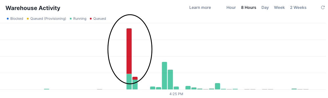
Job Duration Impact:

The sf_export job saw consistent ~10 minute reductions across clients. More importantly, downstream jobs that consume these Parquet files also got faster, without any changes to their code.

Memory Consumption: No Surprises

One concern we had with larger files and different data layouts: would we significantly increase memory consumption?

We filtered out pipelines with high variance (>50% relative standard deviation) to get a clean comparison. The result: memory consumption remained stable. We're not trading memory for speed—we're just using I/O more efficiently.

DuckDB vs. Polars: How They Read Parquet from S3

Since we're using both DuckDB and Polars in our feature computation layer, we've developed a deeper understanding of how each engine approaches Parquet reading—and why our optimizations affected them differently.

How DuckDB Reads Parquet from S3

DuckDB uses its `httpfs` extension for S3 access. Here's what happens when you run a query:

import duckdb

conn = duckdb.connect()
conn.execute("INSTALL httpfs; LOAD httpfs;")

# DuckDB's read path:
result = conn.execute("""
    SELECT entity_id, SUM(value)
    FROM read_parquet('s3://bucket/path/**/*.parquet')
    WHERE market_id = 'abc123'
    GROUP BY entity_id
""").fetchdf()

Under the hood:

1. Metadata fetch: DuckDB first reads just the Parquet footer (last few KB) to get schema and row group metadata
2. Row group pruning: Using min/max statistics from metadata, DuckDB identifies which row groups could possibly contain `market_id = 'abc123'`
3. Column pruning: Only `entity_id`, `value`, and `market_id` columns are fetched—other columns never leave S3
4. Streaming execution: Data streams through the query engine without materializing the full dataset in memory
5. Parallel fetches: Multiple row groups fetched concurrently from S3

DuckDB's approach is pull-based: it reads exactly what the query needs, when it needs it.

How Polars Reads Parquet from S3

Polars takes a different approach with its lazy evaluation model:

import polars as pl

# Polars' read path:
result = (
    pl.scan_parquet("s3://bucket/path/**/*.parquet")
    .filter(pl.col("market_id") == "abc123")
    .group_by("entity_id")
    .agg(pl.col("value").sum())
    .collect()
)

Under the hood:

1. Query plan construction: `scan_parquet()` returns immediately—no data read yet
2. Optimization pass: Before any I/O, Polars' query optimizer analyzes the full query plan
3. Predicate pushdown: The optimizer pushes `market_id = 'abc123'` down to the scan level
4. Projection pushdown: Only required columns marked for retrieval
5. Execution: On `.collect()`, optimized plan executes with parallel S3 fetches

Polars' approach is plan-first: it builds a complete execution plan, optimizes it, then executes.

Why Our Optimizations Affected Them Differently

This is the key insight: the same data layout changes had different effects on different query patterns.

Why Polars showed mixed results:

Our partition changes reduced the number of files from thousands to dozens. Polars' parallelization strategy adapted differently than DuckDB's:

• Polars' parallel strategy: Polars automatically chooses to parallelize across whichever dimension is larger (columns, row groups, or files)
• Before: Many small files with few row groups each → file-level parallelism dominated
• After: Fewer large files with many row groups each → row-group parallelism should dominate, but the optimizer's heuristics for specific query patterns (particularly feature engineering with complex window functions) didn't adapt as effectively as DuckDB's streaming approach

The key insight is that Polars' query optimizer makes upfront decisions about parallelization strategy based on metadata, while DuckDB's streaming execution adapts more dynamically during query processing.

Why DuckDB improved consistently:

DuckDB's streaming execution adapts more dynamically to data layout. Its row-group-level parallelism works regardless of file count. Whether you have 100 files with 10 row groups each or 10 files with 100 row groups each, DuckDB parallelizes at the row group level.

When to Use Each

Based on our production experience:

Choose DuckDB when:

• SQL is your team's primary language
• Complex analytical queries dominate (CTEs, window functions, multi-way joins)
• Memory constraints are tight (DuckDB's streaming execution shines)
• You need consistent performance across varied query patterns

Choose Polars when:

• DataFrame operations fit your mental model better
• You're building ML pipelines that mix transforms with model code
• Your queries are more uniform (Polars' optimizer excels with predictable patterns)
• You want native Rust performance for pure DataFrame operations

Our architecture: We use DuckDB for the analytical heavy lifting (reading from S3, complex joins, aggregations) and Polars for downstream DataFrame manipulations and feature transformations. This hybrid approach lets each engine do what it's best at.

The Takeaway

Don't assume benchmark results transfer to your use case. The interaction between:

• Your data layout (partitioning, sorting, file sizes)
• Your query patterns (filters, joins, aggregations)
• Your engine's optimizer assumptions

...creates unique performance characteristics. Test both engines on YOUR actual workloads with YOUR actual data.

The official Polars benchmarks and community comparisons provide useful baselines, but your mileage will vary.

Implementation Checklist

Ready to apply these optimizations to your own Parquet exports? These changes can be implemented incrementally without requiring infrastructure changes or application rewrites. Start with the audit step to understand your current state, then apply optimizations one at a time to measure their individual impact.

Prerequisites: Access to your Snowflake COPY INTO statements and downstream query patterns.

Here's your step-by-step implementation guide:

1. Audit Your Current State

Count your files. If you have thousands of tiny files, you have a problem.

-- Check your current file sizes in S3
SELECT split_part(metadata$filename, '/', -1) as filename,
       metadata$file_row_number               as rows_in_file
FROM @your_stage/your_path/
LIMIT 100;

2. Identify Your Filter Columns

Review your downstream queries. What columns appear in `WHERE` clauses most frequently? Those are your candidates for`ORDER BY`.

3. Modify Your COPY Statement

COPY INTO 's3://your-bucket/your-path/'
    FROM (
    SELECT
    -- Explicit column list with proper types
    CAST(entity_id AS BIGINT) AS entity_id,
    event_timestamp::TIMESTAMP_NTZ AS event_timestamp,
    metric_value::DOUBLE AS metric_value
    -- ... other columns
    FROM source_table
    ORDER BY entity_id, event_timestamp -- Your primary filter columns
    )
    PARTITION BY ('partition_key=' || partition_column)
    FILE_FORMAT = (TYPE = parquet COMPRESSION = SNAPPY USE_LOGICAL_TYPE = TRUE)
    MAX_FILE_SIZE = 256000000 -- 256 MB

Key Takeaways

On Parquet Optimization

1. Don't throw compute at I/O problems. Before scaling up infrastructure, check if your data layout is sabotaging your readers.
2. Predicate pushdown requires sorted data. Random row distribution makes statistics useless. Add a smart ORDER BY on your filter columns.
3. File size matters. The small file problem is real. Target 128-256 MB minimum for analytical workloads.
4. Partition thoughtfully. Only partition by columns you actually filter on. Over-partitioning recreates the small file problem

On Benchmarking

5. Test both DuckDB and Polars. They respond differently to the same optimizations. Your query patterns determine the winner.
6. Benchmark with production data. Synthetic tests miss real-world patterns. Use your actual feature engineering queries.

References

1. Apache Parquet Documentation - parquet.apache.org
2. Snowflake COPY INTO Documentation - docs.snowflake.com
3. Snowflake File Sizing Best Practices - docs.snowflake.com
4. Polars Predicate Pushdown - pola.rs
5. DuckDB Parquet Support - duckdb.org
6. Parquet Performance Tuning - Alex Merced, Data Engineering with Dremio
7. Understanding Predicate Pushdown at Row Group Level - Peter Hoffmann
8. DuckDB vs Polars Performance - codecentric
9. Polars PDS-H Benchmark Results - pola.rs‍
10. Optimising Parquet Reads with Polars - Rho Signal